Data partition
Here, the full matrix is partitioned into smaller sub-matrixes, and bellow is an example of partition A in to 9 sub-matrixes:
\[A = \begin{pmatrix} { A _ { 11 } } & { A _ { 21 } ^ { T }} & { A _ { 21 } ^ { T }}\\ { A _ { 21 } } & { A _ { 22 } } & { A _ { 21 } ^ { T }} \\ { A _ { 31 } } & { A _ { 32 } } & { A _ { 33 } } \end{pmatrix}\]The sub-matrixes are distributed by block row/column cyclic data distribution. There are two ways of distribution in my algorithm:
- The same rows go to the same rank, row cyclic: $rank( A _{ij} ) = i \mod{n_p}$
- The same columns go the same rank: $rank( A _{ij} ) = j \mod{n_p}$
Where $n_p$ is the number of processors and $A _{ij}$ is the sub-matrix.
The algorithms
By the Cholesky decomposition, for a symmetric positive define matrix , we have
\[A = L L^T = \begin{pmatrix} { A _ { 11 } } & { A _ { 21 } ^ { T }} & &{ A _ { 21 } ^ { T }}\\ { A _ { 21 } } & { A _ { 22 } } & &{ A _ { 21 } ^ { T }} \\ &&...&\\ { A _ { n1 } } & { A _ { n2 } } & &{ A _ { nn } } \end{pmatrix} = \begin{pmatrix} { L _ { 11 } } & && \\ { L _ { 21 } } & { L _ { 22 } } && \\ &&...&\\ { L _ { n1 } } & { L _ { n2 } } && { L _ { nn } } \end{pmatrix} \begin{pmatrix} { L _ { 11 } ^T} & { L _ { 21 } }^T && { L _ { n1} ^T} \\ & { L _ { 22 } }^T & & { L _ { n2 } ^T} \\ &&...&\\ & & &{ L _ { nn }^T } \end{pmatrix}\]And
\(L_{jj} = chol( A _{ij} )\)\(L_{ij}=(A_{ij} - \sum_{k=1}^{j-1}L_{ik}L_{jk}^T)L_{jj}^{-T}\)
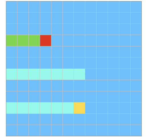
Where $chol( A _{ij} )$ is the lower triangular matrix of Cholesky decomposition of $A _{ij}$, which will be executed in a process sequentially. Below is the data dependency, the red cell lying at diagonal depends on all its left cells(green). The yellow inner cells depend on all its left cells and those whose row number is the same as its column number. Those are colored in light blue.
There are two variants of block-based parallel Cholesky decomposition algorithm: Left-looking and Right-looking.
Right-looking algorithm
Two algorithm proceeds columns by columns, and the computing for column $j$ will start after the column $j-1$ finishes.
\[A = \begin{pmatrix} { A _ { 11 } } &|& & \\ --&&--&--\\ { A _ { 21 } } &|& { A _ { 22 } } &\\ { A _ { 31 } } &|& { A _ { 32 } } & { A _ { 33 } } \end{pmatrix}\]Suppose row 1 $(A_{11} , A_{22}, A_{33})$ has been computed, then
\[A_{22} = chol( A _{22} ) \\ A_{32}=A_{32} A_{22}^{-T} \\ A_{33}=A_{33} - A_{32}A_{32}^{-T}\]The provided sample sequential algorithm is using the right looking way. We can see that the right-looking algorithm requires matrix multiplication between $A_{jj}$to all other sub-matrixes in the same column. As a result, partitioning in the column cyclic way is nature in this algorithm.
The right-looking algorithm can be described as following:
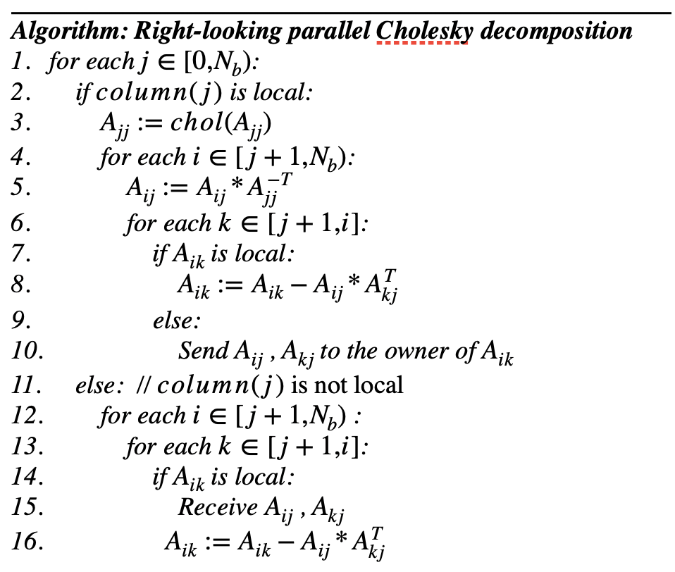
We can see that communication occurs at the innermost loop. The inner loop computation of matrix multiplication and matrix subtract is paralleled on different processors.
Left-looking algorithm
Similar to the right-looking:
\[A = \begin{pmatrix} { A _ { 11 } } &|& & \\ --&&--&--\\ { A _ { 21 } } &|& { A _ { 22 } } &\\ { A _ { 31 } } &|& { A _ { 32 } } & { A _ { 33 } } \end{pmatrix}\]Suppose row 1 $(A_{11} , A_{22}, A_{33})$ has been computed, then \(A_{22}=A_{22} - A_{21}A_{21}^{-T} \\ A_{22} = chol( A _{22} )\\ A_{32}=A_{32} - A_{31} A_{21}^{-T}\\ A_{32} = A_{32}A_{22}^{-T}\)
It is easy to observe that the left-looking algorithm has $A_{jj}$ subtract all is left sub-matrixes’ square. Here I use column cyclic data distribution. Below is the description of the algorithm I wrote:
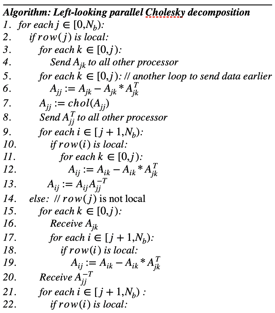
In the left-looking algorithm, the processor has $row(j)$ broadcast all $A_{jj}$’s left matrix and bro broadcast $A_{jj}^T$when $A_{jj}$ is updated. Most communications occur in the second layer loop. I use additional loop to send $A_{jk}$ earlier instead of send $A_{jk} and update $A_{jj}$ in the same loop. For every out-most loop, sub-matrixes in $coloumn(j)$ will be computed in parallel.
Cost Analysis
In right-looking algorithm, the number of message sent in all processors is: \(\sum_{j=0}^{N_b-1}\sum_{i=j+1}^{N_b-1}\sum_{k=j+1}^{i+1} 2 = \frac{N_b^{3}-3N_b^2-4N_b}{3}\) In left-looking, to total number of broadcast is: \(\sum_{j=0}^{N_b-1}\sum_{k=0}^{j-1} = \frac{N_b^{2}-N_b}{2}\) Regarding the $N_p$ amount of unit message(a block) sent in every broadcast call and the time of broadcast is $O(\log N_p)$, left-looking shows lesser communication overhead.
I analyze operations by every round computing column j. And each round is dominated by the processor which owns the column j.
For right-looking, the task is parallels in the inner-most loop. For processor having column j, suppose send blocks until message delivered for simplicity, the time for one inner-most loop is $T_1 = (\frac{O(b^3)}{N_p}+\frac{S(b^2)(N_p-1)}{N_p})$ , where $O(b^3)$ is matrix multiplication (which can be optimized further) for a $b \times b$ block, and $S(b^2)$ is time to send such a block. So as the the rest processors’ inner-most loop, $T_2 = \frac{O(b^3)+S(b^2)}{N_p}$ . Still, inner-most is dominated by the processor having column j. As a result time for round j is: $\sum_{i=j+1}^{N_b-1}\sum_{k=j+1}^{i+1} \max (T_1, T_2)$
For left-looking, the parallel execution demonstrated as following:
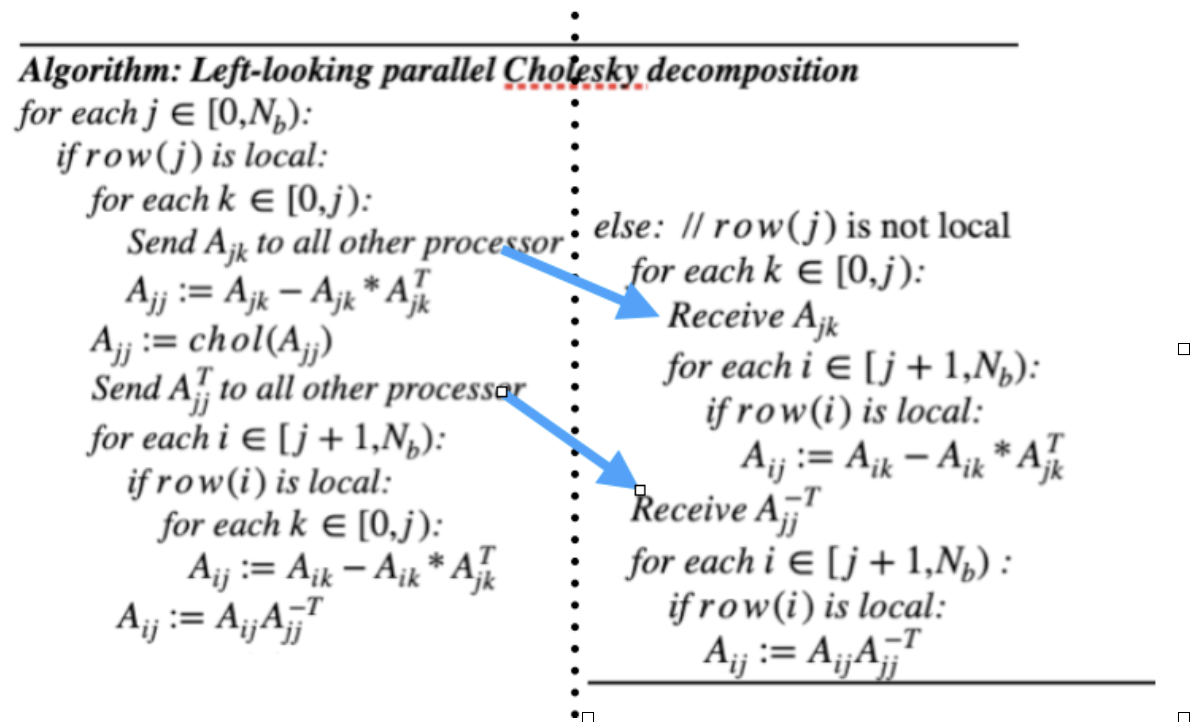
Here the broadcast in left process will not block So total time for round j is
\(T_3 = \sum_{k=0}^{j-1} O(b^3) + \sum_{i=j+1}^{N_b-1} \frac{j O(b^3)}{N_p} = jO(b^3) + (N_b-j-1)\frac{j O(b^3)}{N_p}\), Right process has to wait till $A_{jk}$ received and then do the $A_{ij}$ update, which takes longer and can probably receive $A_{jj}^{-T}$ without any wait. So round j for these processors are
\(T_4 = \sum_{k=0}^{j-1} (S(b^2) + \frac{(N_b-j -1)O(b^3)}{N_p}) + \sum_{i=j+1}^{N_b-1} \frac{ O(b^3)}{N_p} = jS(b^2) + (N_b-j -1)\frac{(j+1)O(b^3)}{N_p}\)
Taking both into account, round time j is $\max(T_3,T_4)$. Note that there is a hidden $O(\log N_p)$ time for broadcast propagation upon the first receive of $A_{jk}$.
From the analysis we can see the computation load balance among processors are similar between these 2 algorithms, but the left-looking algorithm send far less amount of message and numbers of communication.
Implementation
I use C++ to implement the parallel algorithm. The data structure to store a matrix $A_{ij}$ is using STL std::vector<double> instead of c array. As with C array, the memory layout of C++ STL vector is linear and aligned, so there won’t be any performance penalty. The code can be found on github: https://github.com/jaxonwang/parallel_numeric_class/tree/master/a3
The generation of data follows the sample algorithm by calling rand() and let the solution to be $X = (1,1,1,…,1)$. Global full matrix generation is done on rank 0 at first, then distributed by raw/column cyclic way. After data distributed, the full matrix is released to ensure enough memory for rank 0.
I implemented some sequential matrix algorithms which act as basic matrix operations. These sequential can be easily re-written with SIMD or OpenMP for better intra-node parallelism.
Basic matrix computation algorithms
This sequential Cholesky algorithm will be used in the parallel algorithm to update the diagonal sub-matrixes.
void chol_block(vector<double> &a, const int len) {
    int n = len;
    for (int i = 0; i < n; i++) {
        a[i * n + i] = sqrt(a[i * n + i]);
        double invp = 1.0 / a[i * n + i];
        for (int j = i + 1; j < n; j++) {
            a[j * n + i] *= invp;
            for (int k = i + 1; k <= j; k++)
                a[j * n + k] -= a[j * n + i] * a[k * n + i];
        }
    }
}
The matrix inverse is required in the blocked Cholesky decomposition and only needed by the diagonal sub-matrixes that are lower triangular matrix. This operation is $O(n^3)$:
vector<double> trangular_inverse(const vector<double> &A, const int len) {
    vector<double> tmp(A.size(), 0);
    for (int j = 0; j < len; j++) {
        tmp[j * len + j] = 1.0 / A[j * len + j];
        for (int i = j + 1; i < len; i++) {
            double s = 0.0;
            for (int k = j; k < i; k++) {
                s += A[i * len + k] * tmp[k * len + j];
            }
            tmp[i * len + j] = -s / A[i * len + i];
        }
    }
    return tmp;
}
Matrix-matrix multiplication only happens as the form of $AB^T$ , which is cache friendly:
vector<double> A_mul_Bt(const vector<double> &A, const vector<double> &B,
                        const int len) {
    vector<double> C(B.size(), 0);
    for (int i = 0; i < len; i++) {
        for (int j = 0; j < len; j++) {
            double tmp = 0;
            for (int k = 0; k < len; k++) {
                tmp += A[i * len + k] * B[j * len + k];
            }
            C[i * len + j] = tmp;
        }
    }
    return C;
}
All these 3 algorithms exploit the symmetry of matrix to reduce computation.
Right-looking algorithm
void ldlt_rightlooking(const int rank, const int len, const int blk_size,
                       blocks_t &blocks) {
    int block_divided_len = len / blk_size;
    long long Send_num = 0;
    double sendtime = 0;
    double recvtime = 0;
    for (int j = 0; j < block_divided_len; j++) {
        if (get_rank_by_block_id(0, j) == rank) {
            auto &Ajj = get_blocks(blocks, j, j);
            chol_block(Ajj, blk_size);  // Ajj = chol(Ajj)
            auto Ajj_inverse = trangular_inverse(Ajj, blk_size);
            for (int i = j + 1; i < block_divided_len; i++) {
                auto &Aij = get_blocks(blocks, i, j);
                auto newAij =
                    A_mul_Bt(Aij, Ajj_inverse, blk_size);  // Aij = Aij * Ajj_-t
                Aij = move(newAij);
                for (int k = j + 1; k <= i; k++) {
                    int target = get_rank_by_block_id(i, k);
                    auto &Lkj = get_blocks(blocks, k, j);
                    if (target == rank) {  // block is local
                        A_sub_B(get_blocks(blocks, i, k),
                                A_mul_Bt(Aij, Lkj, blk_size),
                                blk_size);  // Aik = Aik - Aij * Akj_t
                    } else {
                        sendtime -= MPI_Wtime();
                        MPI_Send(Aij.data(), Aij.size(), MPI_DOUBLE, target,
                                 Tag::L_matrix, MPI_COMM_WORLD);
                        MPI_Send(Lkj.data(), Lkj.size(), MPI_DOUBLE, target,
                                 Tag::L_matrix, MPI_COMM_WORLD);
                        sendtime += MPI_Wtime();
                        Send_num += 2;
                    }
                }
            }
        } else {
            for (int i = j + 1; i < block_divided_len; i++) {
                for (int k = j + 1; k <= i; k++) {
                    int target = get_rank_by_block_id(i, k);
                    if (target != rank) continue;
                    int source = get_rank_by_block_id(i, j);
                    vector<double> Aij(blk_size * blk_size, 0);
                    vector<double> Lkj(blk_size * blk_size, 0);

                    recvtime -= MPI_Wtime();
                    MPI_Recv(Aij.data(), Aij.size(), MPI_DOUBLE, source,
                             Tag::L_matrix, MPI_COMM_WORLD, MPI_STATUS_IGNORE);
                    MPI_Recv(Lkj.data(), Lkj.size(), MPI_DOUBLE, source,
                             Tag::L_matrix, MPI_COMM_WORLD, MPI_STATUS_IGNORE);
                    recvtime += MPI_Wtime();
                    A_sub_B(get_blocks(blocks, i, k),
                            A_mul_Bt(Aij, Lkj, blk_size),
                            blk_size);  // Aik = Aik - Aij * Akj_t
                }
            }
        }
    }
This function will be called in the main body of all processes. The type blocks_t is defined as:
typedef unordered_map<pair<int, int>, vector<double>> blocks_t;
Variable blocks of type blocks_t stores all local $A_{ij}$ and each processor retrieves its $A_{ij}$ by calling get_blocks(blocks, i, j). It’s retrieved by reference so there is no copy. The storage of blocks_t is not linear, but each block is of the type vector<double>, with careful selection of block size to allow them to fit in the cache. It is worth noting that only the lower triangular matrix will be stored and used in blocks_t.
Left-looking algorithm
void ldlt_leftlooking(const int rank, const int len, const int blk_size,
                      blocks_t &blocks) {
    int block_divided_len = len / blk_size;
    long long Bcast_num = 0;
    double sendtime = 0;
    double recvtime = 0;
    for (int j = 0; j < block_divided_len; j++) {
        int owner = get_rank_by_block_id(j, 0);
        if (owner == rank) {  // if local is owner
            vector<MPI_Request> requests;

            auto &Ajj = get_blocks(blocks, j, j);
            for (int k = 0; k < j; k++) {
                auto &Ajk = get_blocks(blocks, j, k);
                MPI_Request r;
                sendtime -= MPI_Wtime();
                MPI_Ibcast(Ajk.data(), Ajk.size(), MPI_DOUBLE, rank,
                           MPI_COMM_WORLD, &r);
                // MPI_Bcast(Ajk.data(), Ajk.size(), MPI_DOUBLE, owner,
                // MPI_COMM_WORLD);
                sendtime += MPI_Wtime();
                requests.push_back(r);
                Bcast_num++;
            }
            for (int k = 0; k < j; k++) {
                auto &Ajk = get_blocks(blocks, j, k);
                A_sub_B(Ajj, A_mul_Bt(Ajk, Ajk, blk_size),
                        blk_size);  // Ajj -= AjkAjk_t for k: 0~j-1
            }
            chol_block(Ajj, blk_size);
            auto Ajj_inv = trangular_inverse(Ajj, blk_size);
            sendtime -= MPI_Wtime();
            MPI_Request r;
            MPI_Ibcast(Ajj_inv.data(), Ajj_inv.size(), MPI_DOUBLE, rank, MPI_COMM_WORLD,
                       &r);
            // MPI_Bcast(Ajj_inv.data(), Ajj_inv.size(), MPI_DOUBLE, owner,
            // MPI_COMM_WORLD);
            sendtime += MPI_Wtime();
            requests.push_back(r);
            Bcast_num++;
            // if is local
            for (int i = j + 1; i < block_divided_len; i++) {
                if (get_rank_by_block_id(i, j) == rank) {
                    auto &Aij = get_blocks(blocks, i, j);
                    for (int k = 0; k < j; k++) {
                        auto &Aik = get_blocks(blocks, i, k);
                        auto &Ajk = get_blocks(blocks, j, k);
                        A_sub_B(Aij, A_mul_Bt(Aik, Ajk, blk_size),
                                blk_size);  // Aij -= AjkAjk_t for k: 0~j-1
                    }
                    auto newAij = A_mul_Bt(Aij, Ajj_inv, blk_size);
                    Aij = move(newAij);
                }
            }
            MPI_Waitall(requests.size(), requests.data(), MPI_STATUSES_IGNORE);
        } else {  // if not owner
            for (int k = 0; k < j; k++) {
                vector<double> Ajk(blk_size * blk_size, 0.0);
                recvtime -= MPI_Wtime();
                MPI_Request r;
                MPI_Ibcast(Ajk.data(), Ajk.size(), MPI_DOUBLE, owner,
                           MPI_COMM_WORLD, &r);
                MPI_Wait(&r, MPI_STATUSES_IGNORE);
                // MPI_Bcast(Ajk.data(), Ajk.size(), MPI_DOUBLE, owner,
                //           MPI_COMM_WORLD);
                recvtime += MPI_Wtime();
                for (int i = j + 1; i < block_divided_len; i++) {
                    if (get_rank_by_block_id(i, j) == rank) {
                        auto &Aij = get_blocks(blocks, i, j);
                        auto &Aik = get_blocks(blocks, i, k);
                        A_sub_B(Aij, A_mul_Bt(Aik, Ajk, blk_size),
                                blk_size);  // Aij -= AjkAjk_t for k: 0~j-1
                    }
                }
            }
            vector<double> Ajj(blk_size * blk_size, 0);
            recvtime -= MPI_Wtime();
            MPI_Request r;
            MPI_Ibcast(Ajj.data(), Ajj.size(), MPI_DOUBLE, owner,
                       MPI_COMM_WORLD, &r);
            MPI_Wait(&r, MPI_STATUSES_IGNORE);
            // MPI_Bcast(Ajj.data(), Ajj.size(), MPI_DOUBLE, owner,
            // MPI_COMM_WORLD);
            recvtime += MPI_Wtime();
            for (int i = j + 1; i < block_divided_len; i++) {
                if (get_rank_by_block_id(i, j) == rank) {
                    auto &Aij = get_blocks(blocks, i, j);
                    auto newAij = A_mul_Bt(Aij, Ajj, blk_size);
                    Aij = move(newAij);
                }
            }
        }
    }
}
I use the non-blocking broadcast to refrain the process from blocking. After calling MPI_Ibcast(), the matrix will be read by the algorithm, but won’t be written, to ensure it will be correctly broadcasted.
Experiments
Strong scalability
The strong scalability test of both decomposition algorithms are conducted only on a single node of Oakbridge-CX. The size of data here is a square matrix of 16000 dimensions, which is chosen to run both algorithms in 15min. The block size is 32 x 32, which takes 8KB to fit in the L1 cache of one core. I use the Intel MPI compiler with -O3 optimization enabled.
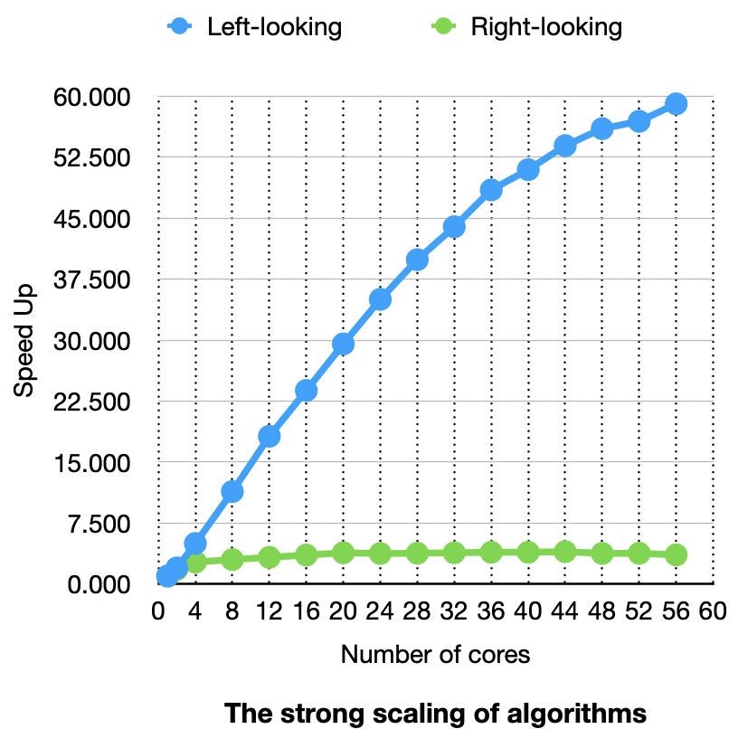
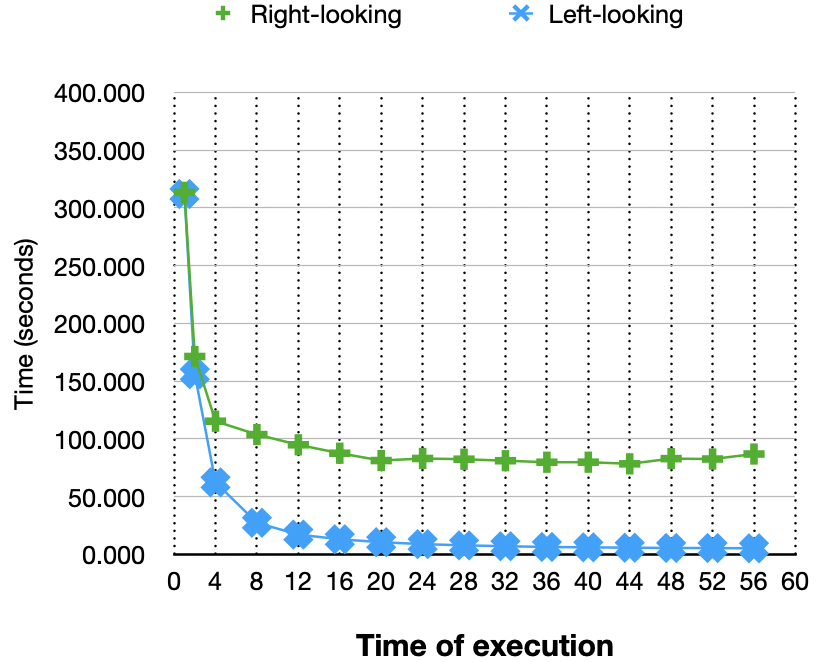
The figure above is the strong scaling of both algorithms. The Speedup is calculated with the sequential baseline by setting the number of processes to 1 in mpiexec. As expected, the left-looking algorithm scales better than the right-looking version. One thing here is the $Speedup(N_p)/N_p$ exceeds 1 in left-looking algorithms. That might be caused by the choice of sequential baseline. The parallel program with parallel degree 1 still divides the whole matrix into sub-matrixes. I choose this to preserve a consistent program behavior. The slope of left looking is close to 1 but slightly goes down when the number of cores is more than 40. Seems the left-looking algorithm scales well in a single node. The right-looking almost does not scale. Below is the execution time of the algorithms:
Weak Scalability
The block size for weak scalability is still 32 x 32 and run on a single node. Unlike weak scalability, I carefully choose the matrix size so that the total operations in the algorithm scales linearly with the number of the cores. The table below shows my choice of data size and the running time results for both algorithms:
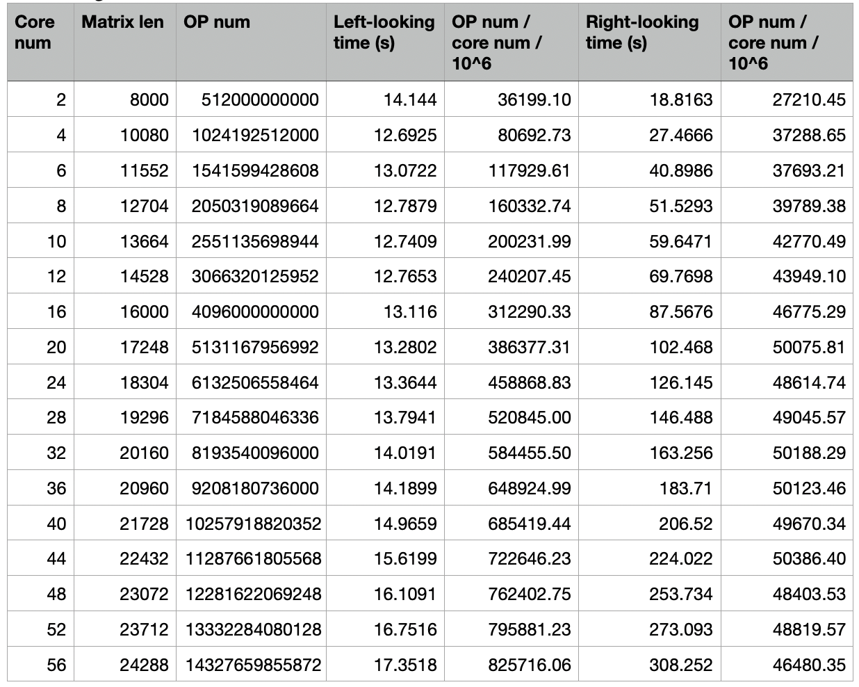
The operation num here is simply the cube of matrix length, it doesn’t present real meaning but can reflect how many operations are done in an algorithm relatively. Below is the weak scalability figure:
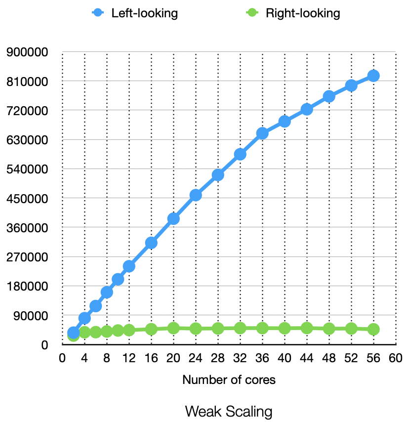
Unsurprisingly, the left-looking algorithm performs better. To have a better view of the right-looking algorithm’s weak scaling:
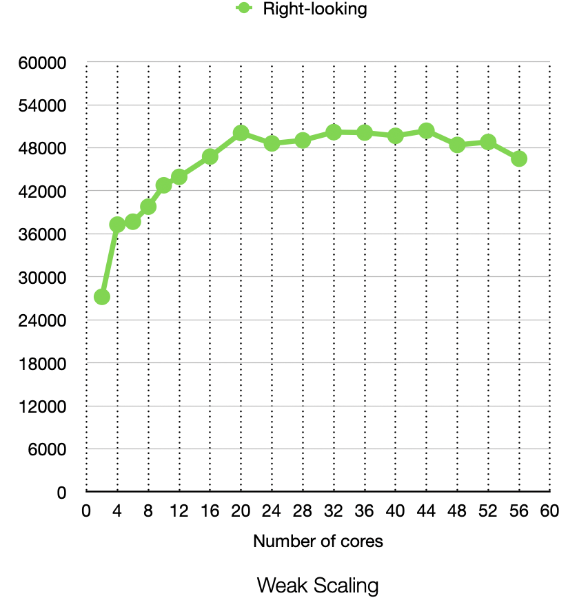
It easy to see that the right-looking slows down when the degree of parallelism goes higher. The reason is due to the cost of communication. Taking matrix length 24288 and number of CPU 56 as an example, below figures demonstrates the performance difference:
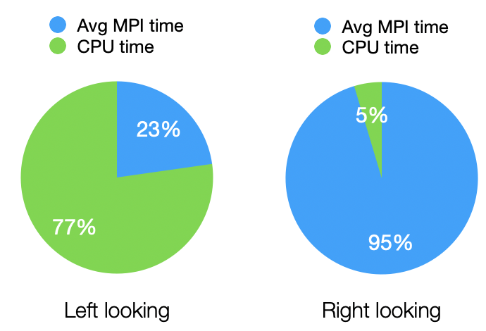 Most time spent on right-looking is communication.
Performance in multi-nodes
The parallel program is tested on a single node since they don’t scale when network communication introduced. Below is the comparison with single-node and 2-node execution with the same data size:

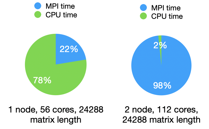
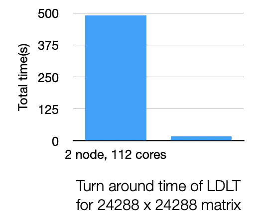
To solve this problem, just replace the basic block Cholesky decomposition and matrix multiplication & inversion & subtraction to in-node parallelism versions implemented by OpenMP and SIMD, but I haven’t implement them in this report.

